1 · Causal vs predictive control under confounding

The one result that motivates chc. Most data science stops at prediction. But a decision changes the future, so it must be judged as an intervention, not a correlation — and chosen by optimal control, not by argmax over a predictive score.

Here we take a confounded offline log (the historical action was targeted at exactly the customers most likely to churn), fit the action's effect two ways, and control the true system with each. The predictive controller drives the system the wrong way; the causal one matches an oracle that knows the true effect.

import jax
import jax.numpy as jnp
import matplotlib.pyplot as plt
import pandas as pd

jax.config.update("jax_enable_x64", True)
jax.config.update("jax_platforms", "cpu")  # the outputs below were made on a CPU
%matplotlib inline

from chc.benchmark import PricingTask
from chc.causal import ConfoundedLinearSystem, estimate_control_effect
from chc.flagship import run_flagship

The confounded log

The data-generating process: a covariate z (customer engagement) drives both the historical action u (a discount) and the outcome x'. Retention teams gave the biggest discounts to the least-engaged customers, the ones most likely to churn, so u falls as z rises. That backdoor path u ← z → x' is what biases a naive fit.

system = ConfoundedLinearSystem()
data = system.sample(20_000, jax.random.key(0))
print("columns:", list(data))
print(
    f"corr(u, z) = {float(jnp.corrcoef(data['u'], data['z'])[0, 1]):+.3f}  "
    "→ the action is entangled with the confounder"
)

columns: ['x', 'z', 'u', 'x_next', 'w']
corr(u, z) = -0.950  → the action is entangled with the confounder

The naive fit flips the sign

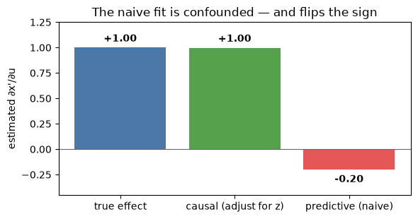
Regress the outcome on the action without adjusting for z (predictive) vs with the adjustment set (causal). The true effect is +1.0.

b_true = system.b_true
b_naive = float(estimate_control_effect(data, adjust_for=()))
b_causal = float(estimate_control_effect(data, adjust_for=("z",)))

effects = pd.DataFrame(
    {"estimate": [b_true, b_causal, b_naive]},
    index=["true effect", "causal (adjust for z)", "predictive (naive)"],
)
effects

	estimate
true effect	1.000000
causal (adjust for z)	0.998507
predictive (naive)	-0.203464

fig, ax = plt.subplots(figsize=(6, 3.2))
colors = ["#4C78A8", "#54A24B", "#E45756"]
ax.bar(effects.index, effects["estimate"], color=colors)
ax.axhline(0, color="0.4", lw=0.8)
ax.set_ylim(-0.45, 1.25)
ax.set_ylabel("estimated ∂x'/∂u")
ax.set_title("The naive fit is confounded — and flips the sign")
for i, v in enumerate(effects["estimate"]):
    ax.text(i, v + (0.06 if v >= 0 else -0.12), f"{v:+.2f}", ha="center", fontweight="bold")
plt.tight_layout()
plt.show()

Control the true system with each estimate

Each controller believes its own estimate and steers the true plant toward a target x* = 2. The predictive controller believes the action lowers the state (b̂ = −0.20). So it pushes the wrong way, as hard as the actuator allows, and the state settles near −20 instead of +2. Without that limit the state would run away. The causal controller reaches the target.

r = run_flagship()
fig, ax = plt.subplots(figsize=(7, 4))
ax.axhline(r["x_target"], ls="--", c="0.5", label="target")
ax.plot(
    r["xs_causal"],
    lw=2.5,
    color="#54A24B",
    label=f"causal control ($\\hat b$ = {r['b_causal']:+.2f})",
)
ax.plot(
    r["xs_naive"],
    lw=2.5,
    color="#E45756",
    label=f"predictive control ($\\hat b$ = {r['b_naive']:+.2f})",
)
ax.set_xlabel("step")
ax.set_ylabel("state x")
ax.set_title("Causal control reaches the target; predictive control settles at −20")
ax.legend()
plt.tight_layout()
plt.show()

print(f"causal final state    = {float(r['xs_causal'][-1]):+.2f}  (target {r['x_target']:+.0f})")
print(f"predictive final state = {float(r['xs_naive'][-1]):+.2f}  ← catastrophe")

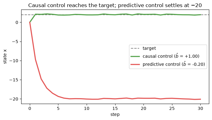
causal final state    = +1.98  (target +2)
predictive final state = -20.09  ← catastrophe

The benchmark: regret vs an oracle

chc ships a benchmark of confounded / constrained / shifting tasks with ground-truth interventional effects, so we can measure regret against an oracle (a controller that knows the true effect), plus constraint violations and out-of-support action rate. PricingTask scores the closed loop above: the same logs, the same noise. regret is a controller's cost above the oracle's. constraint_viol is the share of steps where the state leaves the safe set |x| ≤ 6. ood_rate is the share of actions outside the 1–99 % range of the logged actions.

results = PricingTask().run()
board = pd.DataFrame(
    [
        {
            "controller": r.controller,
            "cost": r.cost,
            "regret": r.regret,
            "constraint_viol": r.constraint_violations,
            "ood_rate": r.ood_rate,
        }
        for r in sorted(results, key=lambda r: r.regret)
    ]
).set_index("controller")
board.round(2)

	cost	regret	constraint_viol	ood_rate
controller
oracle	4.61	0.00	0.00	0.0
causal-CHC	4.61	0.00	0.00	0.0
predictive	13736.84	13732.23	0.97	1.0

Read it off the table: causal-CHC matches the oracle (regret ≈ 0, no constraint violations, no out-of-support actions), while predictive is catastrophic on every axis — huge regret, violates the safe-state constraint most of the time, and acts entirely outside the logged support.

Takeaway

Prediction ≠ decision. Under confounding, optimising control against a predictive model is not just suboptimal — it can be actively harmful. chc makes the causal + control step a first-class object.