7 · Does the gap bite on real data? — the LaLonde validation
Every earlier notebook is synthetic: I made the confounding true, so of course causal beats predictive. The fair test is real data with an experimental ground truth, so the causal estimate can be checked, not asserted. The canonical such dataset is LaLonde's National Supported Work (NSW) job- training experiment (Dehejia–Wahba subset):
- a randomised trial gives the true effect of the program on 1978 earnings (the benchmark);
- a non-experimental version swaps the randomised controls for a survey comparison group (CPS), reproducing the confounding a real observational analyst faces.
This validates the identification core of CHC — the part that decides what effect feeds the controller. (The control loop itself is still the synthetic demo; here we stress-test the causal claim it rests on.) Provenance: R. Dehejia & S. Wahba (2002), data via NBER; nothing is committed to the repo.
import pathlib
import urllib.request

import jax
import jax.numpy as jnp
import matplotlib.pyplot as plt
import pandas as pd

jax.config.update("jax_enable_x64", True)
jax.config.update("jax_platforms", "cpu")  # the outputs below were made on a CPU
%matplotlib inline

from chc.causal import dml_point_and_se, estimate_control_effect, estimate_effect_dml

DATA = pathlib.Path("data")
DATA.mkdir(exist_ok=True)


def load(name: str) -> pd.DataFrame:
    """Load a Dehejia-Wahba .dta, downloading to a local (git-ignored) cache on first use."""
    path = DATA / f"{name}.dta"
    if not path.exists():
        urllib.request.urlretrieve(f"http://users.nber.org/~rdehejia/data/{name}.dta", path)
    return pd.read_stata(path)


COV = ["age", "education", "black", "hispanic", "married", "nodegree", "re74", "re75"]
experimental = load("nsw_dw")  # randomised: NSW treated + randomised controls
cps = load("cps_controls")  # a survey comparison group (the confounding)
for df in (experimental, cps):  # earnings in $1000s keeps the numbers (and DML polynomials) sane
    df[["re74", "re75", "re78"]] /= 1000.0


def to_chc(df: pd.DataFrame) -> dict:
    """Pack a frame into the column dict chc.causal expects (u = treatment, x_next = outcome)."""
    d = {"u": jnp.asarray(df.treat.values, float), "x_next": jnp.asarray(df.re78.values, float)}
    d["x"] = jnp.asarray(df.age.values, float)  # the always-included base regressor
    for c in COV:
        d[c] = jnp.asarray(df[c].values, float)
    return d
The experimental benchmark (ground truth)
Because treatment was randomised, a plain difference in mean 1978 earnings is already unbiased. It is still an estimate from a few hundred men, so it carries a standard error of its own.
treated = experimental.loc[experimental.treat == 1, "re78"]
controls = experimental.loc[experimental.treat == 0, "re78"]
truth = float(treated.mean() - controls.mean())
truth_se = float((treated.var() / len(treated) + controls.var() / len(controls)) ** 0.5)
print(f"experimental ATT (randomised, difference in means) = {truth * 1000:+,.0f} $/yr")
print(
    f"  95% interval {(truth - 1.96 * truth_se) * 1000:+,.0f} to "
    f"{(truth + 1.96 * truth_se) * 1000:+,.0f} $/yr (standard error {truth_se * 1000:,.0f})"
)
print(f"  {len(treated)} treated vs {len(controls)} randomised controls")
experimental ATT (randomised, difference in means) = +1,794 $/yr
  95% interval +479 to +3,109 $/yr (standard error 671)
  185 treated vs 260 randomised controls
The observational trap: a comparison group that isn't comparable
Now replace the randomised controls with the CPS survey group — what an analyst without an experiment would use. The groups differ sharply on almost every covariate: the CPS men are older, more educated, more often married, less often Black, more often finished high school, and earned far more before the program. Only the Hispanic share is similar: 6 % of the NSW men against 7 % of the CPS men. So any naive contrast confounds the program with these gaps.
obs = pd.concat([experimental[experimental.treat == 1], cps], ignore_index=True)
balance = obs.groupby("treat")[COV].mean().rename(index={0: "CPS comparison", 1: "NSW treated"})
balance.round(2)
| age | education | black | hispanic | married | nodegree | re74 | re75 | |
|---|---|---|---|---|---|---|---|---|
| treat | ||||||||
| CPS comparison | 33.23 | 12.03 | 0.07 | 0.07 | 0.71 | 0.30 | 14.02 | 13.65 |
| NSW treated | 25.82 | 10.35 | 0.84 | 0.06 | 0.19 | 0.71 | 2.10 | 1.53 |
Naive vs causal — checked against the truth
- naive (difference in means): what a predictive/associational read of the logs says;
- OLS-adjusted (
estimate_control_effect): linear backdoor adjustment for the covariates; - Double ML (
dml_point_and_se): predict both earnings and treatment from the covariates with flexible (polynomial) models, each fitted on the other folds of the data (cross-fitting). Then regress the earnings the covariates do not explain on the treatment they do not explain. Small errors in the two predictions barely move this residual-on-residual estimate, so it is the estimator meant to survive this kind of imbalance. It also returns a standard error.
obs_chc = to_chc(obs)
naive = float(obs.loc[obs.treat == 1, "re78"].mean() - obs.loc[obs.treat == 0, "re78"].mean())
ols_adj = float(estimate_control_effect(obs_chc, adjust_for=tuple(COV[1:])))
dml, dml_se = dml_point_and_se(obs_chc, covariates=tuple(COV), degree=2, folds=5, ridge=1.0)
# the folds are a random split; refit with ten fold seeds to see how far the point moves
dml_by_seed = [
    float(estimate_effect_dml(obs_chc, covariates=tuple(COV), degree=2, folds=5, ridge=1.0, seed=s))
    for s in range(10)
]
print(
    f"Double ML: standard error {dml_se * 1000:,.0f} $/yr; over fold seeds 0-9 the point runs "
    f"from {min(dml_by_seed) * 1000:+,.0f} to {max(dml_by_seed) * 1000:+,.0f} $/yr"
)

table = pd.DataFrame(
    {"estimate ($/yr)": [truth * 1000, naive * 1000, ols_adj * 1000, dml * 1000]},
    index=[
        "experimental TRUTH",
        "naive (predictive)",
        "OLS-adjusted (CHC)",
        "Double ML (CHC)",
    ],
).round(0)
table["error vs truth"] = table["estimate ($/yr)"] - round(truth * 1000)
table
Double ML: standard error 634 $/yr; over fold seeds 0-9 the point runs from +1,385 to +1,520 $/yr
| estimate ($/yr) | error vs truth | |
|---|---|---|
| experimental TRUTH | 1794.0 | 0.0 |
| naive (predictive) | -8498.0 | -10292.0 |
| OLS-adjusted (CHC) | 699.0 | -1095.0 |
| Double ML (CHC) | 1502.0 | -292.0 |
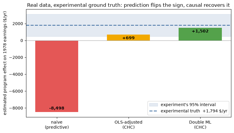
The naive observational estimate is the wrong sign — it says the program destroyed about \$8,500/yr of earnings. A decision driven by that predictive read ("kill the program") would be exactly backwards. CHC's backdoor adjustment restores the correct sign but lands 1,095 below the truth, and Double ML lands 292 below it on the same confounded data. Both estimates fall inside the experiment's own 95 % interval, +479 to +3,109 per year: with 445 men in the experiment, the benchmark itself is uncertain by more than either gap.
fig, ax = plt.subplots(figsize=(8, 4.6))
methods = ["naive\n(predictive)", "OLS-adjusted\n(CHC)", "Double ML\n(CHC)"]
vals = [naive * 1000, ols_adj * 1000, dml * 1000]
colors = ["#E45756", "#F2A900", "#54A24B"]
lo, hi = (truth - 1.96 * truth_se) * 1000, (truth + 1.96 * truth_se) * 1000
ax.axhspan(lo, hi, color="#4C78A8", alpha=0.15, label="experiment's 95% interval")
ax.axhline(
    truth * 1000,
    color="#4C78A8",
    lw=2,
    ls="--",
    label=f"experimental truth  {truth * 1000:+,.0f} $/yr",
)
ax.axhline(0, color="0.6", lw=0.8)
bars = ax.bar(methods, vals, color=colors, width=0.6)
for b, v in zip(bars, vals, strict=True):  # label inside the bar's end, clear of the truth line
    ax.annotate(
        f"{v:+,.0f}",
        (b.get_x() + b.get_width() / 2, v),
        xytext=(0, -4 if v > 0 else 4),
        textcoords="offset points",
        ha="center",
        va="top" if v > 0 else "bottom",
        fontweight="bold",
    )
ax.set_ylabel("estimated program effect on 1978 earnings ($/yr)")
ax.set_title("Real data, experimental ground truth: prediction flips the sign, causal recovers it")
ax.legend(loc="lower right")
plt.tight_layout()
plt.show()
Takeaway — the honest answer to "is this real?"
Yes, the gap bites on real data. On the LaLonde NSW data the predictive/associational estimate is not merely biased — it has the wrong sign, and a decision made from it would be the opposite of correct. CHC's causal estimators restore the sign from the confounded observational data: adjustment lands 1,095 below the randomised truth, and Double ML lands 292 below it.
Scope, stated honestly: this validates the identification half of CHC — the effect that feeds the
controller — on real data with a checkable ground truth. It does not by itself validate the control
loop on real dynamics (that remains the synthetic demo). The Double ML number depends on the nuisance
learner (here degree-2 polynomials) and on the random fold split: ten fold seeds move it from
+1,385 to +1,520. The benchmarks page runs the same rows through chc.lalonde, which
standardises the covariates and fits degree-3 nuisances: its OLS row matches the one here, and its
Double ML row differs. Both regressions also estimate a variance-weighted average of the effect, not
the effect on the treated that the experiment measures; the two coincide if the effect is the same
for everyone. What it does settle: the load-bearing premise of the whole library — use the
intervention, not the prediction, to make the decision — is real, and expensive to ignore.