4 · Scientific control & offline safety

Two more advantages of chc on realistic control problems:

1. Constrained optimal control on nonlinear scientific dynamics — flatten an epidemic curve under a hospital-capacity constraint with minimal intervention (nonlinear population models with optimal control, in the tradition of Bazykin, Riznichenko and Marchuk).
2. Offline safety via pessimism — a controller trained offline must not exploit its model where it was never trained; the pessimism/support layer keeps actions inside the region the data justifies.

import jax
import jax.numpy as jnp
import matplotlib.pyplot as plt
import pandas as pd

jax.config.update("jax_enable_x64", True)
jax.config.update("jax_platforms", "cpu")  # the outputs below were made on a CPU
%matplotlib inline

from chc.benchmark import SupportShiftTask
from chc.epidemic import SIRDynamics, optimal_npi
from chc.integrate import rollout

Flatten the curve: SIR + NPI under a capacity constraint

A fast epidemic (R₀ = 6: while everyone is susceptible, each case infects six others) overshoots hospital capacity. optimal_npi finds the least intervention (a non-pharmaceutical-intervention schedule reducing transmission) that holds infections at the cap. It minimises the sum of squared daily intensities plus a steep penalty on infections above the cap, by projected-gradient optimal control that differentiates through the rollout. Because the cap is a penalty, not a hard limit, the controlled peak ends just above it. The schedule ramps up before infections reach the cap, eases off as the pool of susceptible people shrinks, and stops once the epidemic can no longer grow.

model = SIRDynamics(beta=0.6, gamma=0.1)  # R0 = 6
x0 = jnp.array([0.99, 0.01])
dt, horizon, i_max = 1.0, 100, 0.1

xs_free = rollout(model, x0, jnp.zeros((horizon, 1)), dt)
us = optimal_npi(model, x0, dt, horizon, i_max)
xs_ctrl = rollout(model, x0, us, dt)

fig, ax = plt.subplots(figsize=(7.5, 4))
ax.axhline(i_max, ls="--", c="0.5", label="hospital capacity")
ax.plot(xs_free[:, 1], lw=2.5, color="#E45756", label="no intervention")
ax.plot(xs_ctrl[:, 1], lw=2.5, color="#54A24B", label="optimal NPI")
ax.plot(us[:, 0], lw=1.2, ls=":", color="#4C78A8", label="NPI intensity u")
ax.set_xlabel("day")
ax.set_ylabel("infected fraction I  /  NPI intensity u")
ax.set_title("Flatten the curve: least-intervention control under a capacity cap")
ax.legend()
plt.tight_layout()
plt.show()

print(f"uncontrolled peak I = {float(jnp.max(xs_free[:, 1])):.4f}   (cap {i_max})")
print(f"controlled   peak I = {float(jnp.max(xs_ctrl[:, 1])):.4f}   flattened to the cap")
print(f"sum of daily NPI intensities = {float(jnp.sum(us)):.1f}")

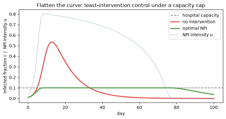
uncontrolled peak I = 0.5358   (cap 0.1)
controlled   peak I = 0.1004   flattened to the cap
sum of daily NPI intensities = 44.0

Offline safety: pessimism vs a greedy controller

Here the model is linear and exact on the logged actions, but the true plant's control effectiveness collapses off-support (a real actuator has a sweet spot). The greedy controller extrapolates to large actions to chase the gains the model promises — and stalls on the true plant. Pessimism adds a penalty that grows with each state–action pair's distance from the centre of the logged data. So the pessimistic controller keeps its actions inside the offline support, where the model is right. The oracle plans on the true plant.

results = SupportShiftTask().run()
board = pd.DataFrame(
    [
        {
            "controller": r.controller,
            "true cost": r.cost,
            "regret vs oracle": r.regret,
            "out-of-support rate": r.ood_rate,
        }
        for r in sorted(results, key=lambda r: r.regret)
    ]
).set_index("controller")
board.round(2)

	true cost	regret vs oracle	out-of-support rate
controller
oracle	20.65	0.00	0.0
pessimistic	22.89	2.24	0.0
greedy	28.01	7.36	0.4

by = {r.controller: r for r in results}
fig, ax = plt.subplots(figsize=(6.5, 3.6))
names = ["oracle", "pessimistic", "greedy"]
regrets = [by[n].regret for n in names]
oods = [by[n].ood_rate for n in names]
xpos = range(len(names))
ax.bar(xpos, regrets, color=["#4C78A8", "#54A24B", "#E45756"])
ax.set_xticks(list(xpos))
ax.set_xticklabels(names)
ax.set_ylabel("regret vs oracle")
ax.set_title("Pessimism avoids the model-exploitation cliff")
for i, (rg, od) in enumerate(zip(regrets, oods, strict=True)):
    ax.text(i, rg + 0.1, f"regret {rg:.1f}\n{od:.0%} OOD", ha="center", va="bottom", fontsize=9)
ax.set_ylim(0, max(regrets) * 1.35)
plt.tight_layout()
plt.show()

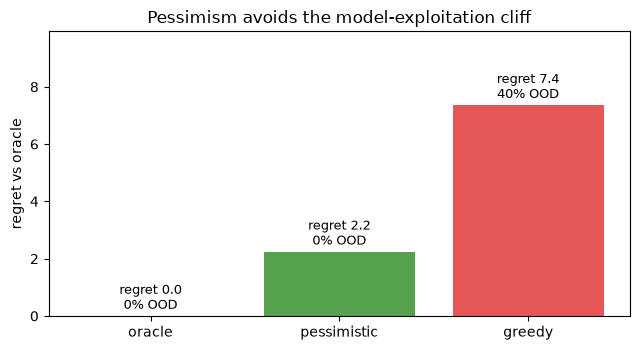
The greedy controller pushes a large fraction of its actions out of the logged support and pays for it in regret; pessimism keeps every action in-support and cuts the regret to about a third (2.2 against 7.4). Here the safeguard is pessimism, not causality — the two failure modes (confounding and off-support model error) are independent, and chc addresses both.

Takeaway

chc does constrained optimal control on genuine nonlinear dynamics, and its offline-safety layer stops an offline-trained controller from exploiting model error where the data cannot back it up.