3 · The causal inference toolkit¶

For control we need the interventional effect ∂x′/∂do(u), not a correlation. chc ships a small, self-contained causal layer that goes well beyond a naive regression:

tool	when to use
adjustment	the confounder is observed → block the backdoor path
IV / 2SLS	the confounder is latent but you have an instrument
Double ML	confounding is nonlinear (linear adjustment is biased)
sensitivity	quantify how much hidden confounding your decision tolerates
refutation	placebo / random-cause / subset robustness checks

(For heavier estimators chc wraps other libraries instead of reimplementing them. chc.estimators.EconMLDoubleML takes any EconML DML estimator that fits on outcome, treatment and covariates, such as CausalForestDML. chc.estimators.DoWhyEstimator runs DoWhy's identify-then-estimate workflow. Neither library is a chc dependency.)

import jax
import matplotlib.pyplot as plt
import pandas as pd

jax.config.update("jax_enable_x64", True)
jax.config.update("jax_platforms", "cpu")  # the outputs below were made on a CPU
%matplotlib inline

from chc.causal import (
    ConfoundedLinearSystem,
    estimate_control_effect,
    estimate_effect_dml,
    estimate_effect_iv,
    refute_effect,
    sensitivity_analysis,
)

1 · Adjustment: block the backdoor¶

When the confounder z is observed, conditioning on it recovers the true effect (+1.0); omitting it leaves a confounded — here sign-flipped — estimate.

data = ConfoundedLinearSystem().sample(20_000, jax.random.key(0))
pd.DataFrame(
    {
        "estimate": [
            1.0,
            float(estimate_control_effect(data, adjust_for=("z",))),
            float(estimate_control_effect(data, adjust_for=())),
        ]
    },
    index=["true", "adjusted (causal)", "unadjusted (naive)"],
).round(3)

	estimate
true	1.000
adjusted (causal)	0.999
unadjusted (naive)	-0.203

2 · Instrumental variables: a latent confounder¶

If z is unobserved we cannot adjust for it. But an instrument w (it drives the action, is independent of the confounder, and only affects the outcome through the action) identifies the effect via two-stage least squares.

iv_data = ConfoundedLinearSystem(gamma=1.0).sample(40_000, jax.random.key(0))  # instrument active
pd.DataFrame(
    {
        "estimate": [
            1.0,
            float(estimate_control_effect(iv_data, adjust_for=())),  # z is latent → biased
            float(estimate_effect_iv(iv_data, instrument="w")),
        ]
    },
    index=["true", "naive (z latent)", "IV / 2SLS (instrument w)"],
).round(3)

	estimate
true	1.000
naive (z latent)	0.140
IV / 2SLS (instrument w)	1.009

3 · Double ML: nonlinear confounding¶

When the confounder enters nonlinearly (here z²), a linear adjustment is biased. Double/debiased ML predicts the outcome and the action from the covariates with a flexible model, subtracts the predictions, and regresses what is left of the outcome on what is left of the action. Each prediction comes from a model fitted on the other half of the data (cross-fitting). Small errors in those predictions then do not bias the effect to first order (Neyman orthogonality). It recovers the effect.

k = jax.random.split(jax.random.key(1), 4)
n = 20_000
x = jax.random.normal(k[0], (n,))
z = jax.random.normal(k[1], (n,))
u = z**2 + jax.random.normal(k[2], (n,))  # action depends nonlinearly on z
y = 0.5 * x + 1.0 * u + 1.5 * z**2 + 0.1 * jax.random.normal(k[3], (n,))  # z² confounding
nl = {"x": x, "z": z, "u": u, "x_next": y}
pd.DataFrame(
    {
        "estimate": [
            1.0,
            float(estimate_control_effect(nl, adjust_for=("z",))),  # linear in z → biased
            float(estimate_effect_dml(nl, covariates=("x", "z"), degree=3)),
        ]
    },
    index=["true", "linear adjust for z", "Double ML (poly nuisances)"],
).round(3)

	estimate
true	1.000
linear adjust for z	2.011
Double ML (poly nuisances)	1.000

4 · Sensitivity: how much hidden confounding would overturn the decision?¶

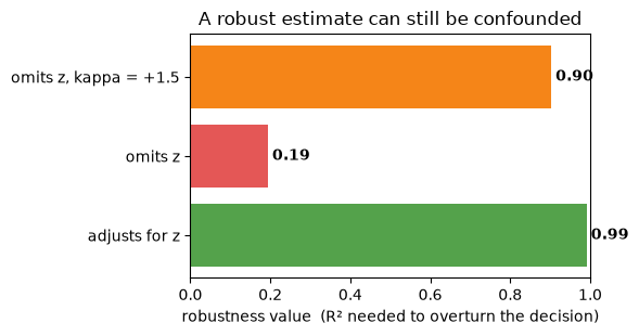
The Cinelli–Hazlett robustness value is the share of the remaining variance (partial R²) that an unobserved confounder would have to explain in both the action and the outcome to drive the estimate to zero. It measures how much hidden confounding an estimate can absorb. It does not tell whether the estimate is confounded. On the IV data of section 2, the estimate that adjusts for z survives a confounder that explains up to 99 %. The estimate that omits z (0.14) is small against its noise, and a confounder that explains 19.5 % would erase it. A confounded estimate can still look robust. The third row omits z on data where the confounder pulls the action up instead of down (kappa = +1.5 against the default −1.5). The confounding then adds to the effect: the naive estimate is 1.86 against a true 1.0, and its robustness value is 0.90.

same_way = ConfoundedLinearSystem(gamma=1.0, kappa=1.5).sample(40_000, jax.random.key(0))
rv = pd.DataFrame(
    [
        sensitivity_analysis(iv_data, adjust_for=("z",)),
        sensitivity_analysis(iv_data, adjust_for=()),
        sensitivity_analysis(same_way, adjust_for=()),
    ],
    index=["adjusts for z", "omits z", "omits z, kappa = +1.5"],
)[["effect", "std_error", "robustness_value"]]
rv.round(4)

	effect	std_error	robustness_value
adjusts for z	0.9998	0.0004	0.9922
omits z	0.1395	0.0032	0.1949
omits z, kappa = +1.5	1.8592	0.0032	0.9036

fig, ax = plt.subplots(figsize=(6, 3.2))
ax.barh(rv.index, rv["robustness_value"], color=["#54A24B", "#E45756", "#F58518"])
ax.set_xlim(0, 1)
ax.set_xlabel("robustness value  (R² needed to overturn the decision)")
ax.set_title("A robust estimate can still be confounded")
for i, v in enumerate(rv["robustness_value"]):
    ax.text(v + 0.01, i, f"{v:.2f}", va="center", fontweight="bold")
plt.tight_layout()
plt.show()

png

5 · Refutation: automatic robustness checks¶

Before trusting an effect, chc runs DoWhy-style refuters: permuting the treatment must collapse the effect (placebo → 0), an irrelevant covariate must not change it (random common cause), and a subsample must reproduce it (subset).

report = refute_effect(data, adjust_for=("z",))
pd.DataFrame({k: [v] for k, v in report.items()}).T.rename(columns={0: "value"})

	value
original	0.998507
placebo	-0.002352
random_common_cause	0.998497
subset	0.997491
passes	True

Takeaway¶

The causal layer is genuinely deep — adjustment, IV, Double ML, sensitivity, and refutation — so the effect that feeds the controller is interventional and stress-tested, not a naive slope.