6 · Adaptive cruise control from confounded fleet logs (a relatable end-to-end)
A concrete, everyday control problem that ties the whole library together. We want adaptive cruise control: hold the car at a target speed by setting the throttle. Our main data are observational fleet logs — no controlled experiment on the throttle — and they are confounded:
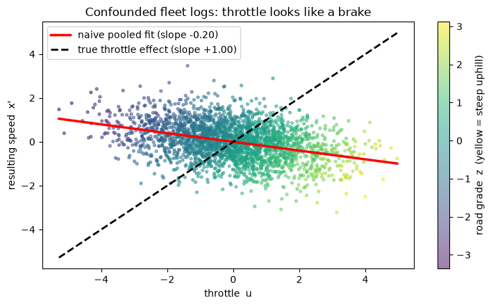
On hills, drivers pressed the throttle harder, yet the car went slower (the grade fought them). So in the raw logs, more throttle correlates with lower speed — as if the throttle were a brake.
A predictive model trained on those logs learns exactly that wrong lesson. Deployed as a cruise
controller, it brakes to speed up and the car stalls. chc recovers the true throttle→speed effect
in either of two ways. If the grade is logged, it adjusts for the grade. If it is not, it uses a
randomised throttle nudge, given to a second fleet, as an instrumental variable (IV). With the
recovered effect, the controller holds speed. Same machinery as notebook 1, in a domain everyone has
felt.
import jax
import jax.numpy as jnp
import matplotlib.pyplot as plt
import numpy as np
import pandas as pd

jax.config.update("jax_enable_x64", True)
jax.config.update("jax_platforms", "cpu")  # the outputs below were made on a CPU
%matplotlib inline

from chc.causal import (
    ConfoundedLinearSystem,
    estimate_control_effect,
    estimate_effect_iv,
    sensitivity_analysis,
)
from chc.flagship import closed_loop

# x = speed (relative to base), u = throttle, z = road grade (the confounder), w = randomised nudge.
# True effect of throttle on next speed is +1.0; grade slows the car (c<0) and drivers gave more
# throttle on steeper grade (kappa>0) — so the naive throttle->speed estimate flips negative.
cruise = ConfoundedLinearSystem(a=0.5, b_true=1.0, c=-2.0, kappa=1.5, gamma=0.0)
logs = cruise.sample(20_000, jax.random.key(0))
The logs look like "throttle slows the car"
Colour each logged step by road grade. Steep-uphill points (yellow) cluster at high throttle but low resulting speed; downhill points (dark purple) sit at low throttle and high speed. The pooled trend line slopes down. Within any single grade band the true relationship is positive — this is Simpson's paradox, and it is a confounded control effect.
idx = jax.random.choice(jax.random.key(1), logs["u"].shape[0], (2500,), replace=False)
u_s, y_s, z_s = (
    np.asarray(logs["u"][idx]),
    np.asarray(logs["x_next"][idx]),
    np.asarray(logs["z"][idx]),
)
# fit the pooled line on all 20,000 steps; plot 2,500 of them so the points stay readable
slope, intercept = np.polyfit(np.asarray(logs["u"]), np.asarray(logs["x_next"]), 1)

fig, ax = plt.subplots(figsize=(7.5, 4.5))
sc = ax.scatter(u_s, y_s, c=z_s, cmap="viridis", s=8, alpha=0.5)
xs_line = np.linspace(u_s.min(), u_s.max(), 2)
ax.plot(
    xs_line,
    slope * xs_line + intercept,
    "r-",
    lw=2.5,
    label=f"naive pooled fit (slope {slope:+.2f})",
)
ax.plot(xs_line, 1.0 * xs_line + intercept, "k--", lw=2, label="true throttle effect (slope +1.00)")
ax.set_xlabel("throttle  u")
ax.set_ylabel("resulting speed  x'")
ax.set_title("Confounded fleet logs: throttle looks like a brake")
plt.colorbar(sc, label="road grade  z  (yellow = steep uphill)")
ax.legend(loc="upper left")
plt.tight_layout()
plt.show()
Estimate the throttle→speed effect three ways
- naive (regress speed on throttle) — confounded, wrong sign;
- adjust for grade — if the grade is logged, conditioning on it blocks the backdoor path
throttle ← grade → speed; - IV — if the grade is not logged, use a second fleet: 40,000 separate steps in which every
throttle got a randomised nudge (instrument
w). Two-stage least squares (2SLS) recovers the effect.
The two regression estimates also get a robustness value: the share of the remaining variance of both throttle and speed that a hidden confounder would need to explain to erase the estimate.
ab_logs = ConfoundedLinearSystem(a=0.5, b_true=1.0, c=-2.0, kappa=1.5, gamma=1.0).sample(
    40_000, jax.random.key(2)
)  # a fleet with a randomised throttle nudge active
estimates = pd.DataFrame(
    {
        "estimate": [
            1.0,
            float(estimate_control_effect(logs, adjust_for=())),
            float(estimate_control_effect(logs, adjust_for=("z",))),
            float(estimate_effect_iv(ab_logs, instrument="w")),
        ],
        "robustness value": [
            np.nan,
            sensitivity_analysis(logs, adjust_for=())["robustness_value"],
            sensitivity_analysis(logs, adjust_for=("z",))["robustness_value"],
            np.nan,
        ],
    },
    index=["true effect", "naive", "adjust for grade (causal)", "IV (randomised nudge)"],
).round(3)
r2_grade = float(jnp.corrcoef(logs["u"], logs["z"])[0, 1] ** 2)
print(f"grade explains {r2_grade:.0%} of the logged throttle's variance")
estimates
grade explains 90% of the logged throttle's variance
| estimate | robustness value | |
|---|---|---|
| true effect | 1.000 | NaN |
| naive | -0.203 | 0.395 |
| adjust for grade (causal) | 0.999 | 0.963 |
| IV (randomised nudge) | 0.994 | NaN |
The naive estimate is negative: throttle "slows" the car. Its robustness value, 0.395, is not small, so this number alone would not flag the problem: a hidden confounder must explain 39.5 % of the remaining variance of both throttle and speed to erase the estimate. Grade is far stronger than that: it explains 90 % of the logged throttle's variance. Adjusting for grade and IV both recover ≈ +1.0; the adjusted estimate's robustness value is 0.963.
Deploy as cruise control: hold +2 above base speed
Plan with each estimate, act on the true car (chc's model/plant split). The causal controller plans
with the grade-adjusted estimate, opens the throttle and holds the setpoint; the predictive controller
— believing throttle is a brake — lifts off / brakes to "gain" speed and the car falls away.
x0, target, n_steps = jnp.asarray(0.0), 2.0, 30
key = jax.random.key(7)
b_naive = float(estimate_control_effect(logs, adjust_for=()))
b_causal = float(estimate_control_effect(logs, adjust_for=("z",)))
xs_causal, us_causal = closed_loop(cruise, b_causal, x0, target, n_steps, -10.0, 10.0, key)
xs_naive, us_naive = closed_loop(cruise, b_naive, x0, target, n_steps, -10.0, 10.0, key)

fig, (ax1, ax2) = plt.subplots(1, 2, figsize=(11, 4))
ax1.axhline(target, ls="--", c="0.5", label="target speed")
ax1.plot(xs_causal, lw=2.5, color="#54A24B", label="causal-CHC (holds speed)")
ax1.plot(xs_naive, lw=2.5, color="#E45756", label="predictive (stalls)")
ax1.set_xlabel("step")
ax1.set_ylabel("speed  x")
ax1.set_title("Speed vs setpoint")
ax1.legend()
ax2.plot(us_causal, lw=2, color="#54A24B", label="causal throttle")
ax2.plot(us_naive, lw=2, color="#E45756", label="predictive throttle")
ax2.axhline(0, c="0.7", lw=0.8)
ax2.set_xlabel("step")
ax2.set_ylabel("throttle  u")
ax2.set_title("The predictive controller brakes to 'speed up'")
ax2.legend()
plt.tight_layout()
plt.show()

err_causal = float(jnp.mean(jnp.abs(xs_causal[1:] - target)))
err_naive = float(jnp.mean(jnp.abs(xs_naive[1:] - target)))
print(
    f"mean |speed - target| over {n_steps} steps — causal: {err_causal:.2f}   "
    f"predictive: {err_naive:.2f}"
)
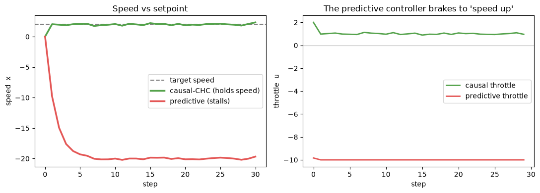
mean |speed - target| over 30 steps — causal: 0.11 predictive: 21.34
Takeaway
Same failure and same fix as notebook 1, in a domain you can feel: prediction learns the confounded association, control needs the intervention. Adjust for the confounder when you can measure it, reach for an instrument when you cannot — then let optimal control do its job on the true system.