2 · Learning what physics misses (hybrid dynamics + system ID)¶

A domain expert can write down most of a system — an RC thermal balance, an orbital force model, a compartmental epidemic — but never all of it. chc models ẋ = f_known(x, u) + r_θ(x, u), a known mechanism plus a learned residual, and trains only the residual, leaving the known physics intact. The known physics carries most of the structure, so a hybrid model can need less data than a black box and extrapolate further. 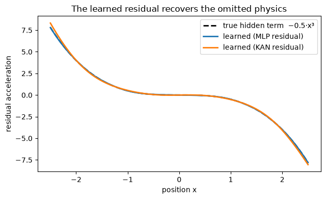It also keeps the learned part small and interpretable, as the plot below shows.

Here the true plant is a damped oscillator plus a hidden cubic stiffening term. The known model omits the cubic; we recover it from data.

import equinox as eqx
import jax
import jax.numpy as jnp
import matplotlib.pyplot as plt
import pandas as pd

jax.config.update("jax_enable_x64", True)
jax.config.update("jax_platforms", "cpu")  # the outputs below were made on a CPU
%matplotlib inline

from chc.dynamics import DampedOscillator, HybridDynamics
from chc.integrate import rk4_step, rollout
from chc.residual import KANResidual, MLPResidual, ZeroResidual
from chc.train import fit_residual, fit_residual_multistep, one_step_mse

DT = 0.05


class CubicResidual(eqx.Module):
    """The hidden physics the known model omits: a cubic stiffening force."""

    beta: float

    def __call__(self, t, x, u):
        return jnp.array([0.0, -self.beta * x[0] ** 3])


known = DampedOscillator(omega=1.0, zeta=0.1)
true_plant = HybridDynamics(known=known, residual=CubicResidual(beta=0.5))

Generate exact (noise-free) one-step transitions from the true plant¶

The actions are drawn at random, independently of the state. That is why fitting by prediction error below recovers the residual. If a policy had chosen the actions from something that also drives the state, prediction error would learn the wrong control response; chc.dynamics_id.fit_causal_residual is the fit for that case.

k_x, k_u = jax.random.split(jax.random.key(0))
xs = jax.random.normal(k_x, (2000, 2))
us = 0.5 * jax.random.normal(k_u, (2000, 1))
x_next = jax.vmap(lambda x, u: rk4_step(true_plant, 0.0, x, u, DT))(xs, us)
data = {"x": xs, "u": us, "x_next": x_next}

known_only = HybridDynamics(known=known, residual=ZeroResidual(out_dim=2))
mse_known = float(one_step_mse(known_only, xs, us, x_next, DT))
print(f"known-only one-step MSE = {mse_known:.4e}  (the residual it ignores)")

known-only one-step MSE = 5.2612e-03  (the residual it ignores)

Fit a residual — MLP and interpretable RBF-KAN backends¶

The residual is interchangeable: the same training code works for an MLP and for a KAN, a Kolmogorov–Arnold network whose edges are one-dimensional curves you can plot.

rows = [("known-only (r=0)", mse_known)]
trained = {}
for name, residual in [
    ("MLP residual", MLPResidual(2, 1, 2, width=32, key=jax.random.key(1))),
    ("KAN residual", KANResidual(2, 1, 2, num_grid=12, grid_range=4.0, key=jax.random.key(2))),
]:
    model, _ = fit_residual(HybridDynamics(known=known, residual=residual), data, DT, steps=2000)
    trained[name] = model
    rows.append((name, float(one_step_mse(model, xs, us, x_next, DT))))

table = pd.DataFrame(rows, columns=["model", "one-step MSE"]).set_index("model")
table["error cut"] = (mse_known / table["one-step MSE"]).map(lambda v: f"{v:,.0f}×")
table

	one-step MSE	error cut
model
known-only (r=0)	5.261207e-03	1×
MLP residual	2.262475e-07	23,254×
KAN residual	3.153087e-05	167×

Both learned residuals cut the one-step error by more than 100× (KAN 167×, MLP over 20,000×) — the hybrid model recovers the physics the known model omits.

The learned residual matches the true hidden physics¶

Because the residual is a small function of x, we can plot it against the ground truth — it learned the cubic, not a black-box blob.

grid = jnp.linspace(-2.5, 2.5, 100)
u0 = jnp.zeros(1)
true_curve = jax.vmap(lambda p: CubicResidual(0.5)(0.0, jnp.array([p, 0.0]), u0)[1])(grid)
fig, ax = plt.subplots(figsize=(6.5, 4))
ax.plot(grid, true_curve, "k--", lw=2, label="true hidden term  −0.5·x³")
for name, model in trained.items():
    learned = jax.vmap(lambda p: model.residual(0.0, jnp.array([p, 0.0]), u0)[1])(grid)
    ax.plot(grid, learned, lw=2, label=f"learned ({name})")
ax.set_xlabel("position x")
ax.set_ylabel("residual acceleration")
ax.set_title("The learned residual recovers the omitted physics")
ax.legend()
plt.tight_layout()
plt.show()

png

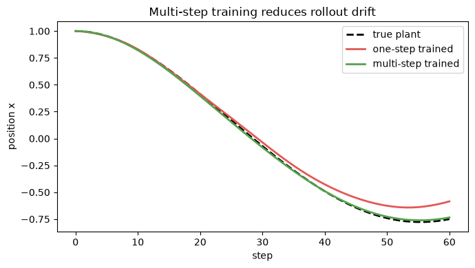
Multi-step training cuts long-horizon drift¶

One-step (teacher-forced) fitting starts each step from the measured state and minimises that step's error. Here every measured state carries noise with standard deviation 0.02. The one-step fit takes each noisy state as exact, and over a long rollout its errors compound. fit_residual_multistep fits whole rollouts instead, each from its first measured state. The last printed line shows the one-step fit on the same trajectories without noise.

horizon, n_traj = 15, 300
k0, k1, k2 = jax.random.split(jax.random.key(3), 3)
x0s = 0.8 * jax.random.normal(k0, (n_traj, 2))
u_seq = 0.3 * jax.random.normal(k1, (n_traj, horizon, 1))
xs_clean = jax.vmap(lambda x0, u: rollout(true_plant, x0, u, DT))(x0s, u_seq)
xs_noisy = xs_clean + 0.02 * jax.random.normal(k2, xs_clean.shape)


def fresh():
    return HybridDynamics(
        known=known, residual=MLPResidual(2, 1, 2, width=32, key=jax.random.key(1))
    )


m_one, _ = fit_residual(
    fresh(),
    {
        "x": xs_noisy[:, :-1].reshape(-1, 2),
        "u": u_seq.reshape(-1, 1),
        "x_next": xs_noisy[:, 1:].reshape(-1, 2),
    },
    DT,
    steps=1500,
)
m_multi, _ = fit_residual_multistep(
    fresh(), {"x0": xs_noisy[:, 0], "us": u_seq, "xs": xs_noisy}, DT, steps=1500
)
m_clean, _ = fit_residual(
    fresh(),
    {
        "x": xs_clean[:, :-1].reshape(-1, 2),
        "u": u_seq.reshape(-1, 1),
        "x_next": xs_clean[:, 1:].reshape(-1, 2),
    },
    DT,
    steps=1500,
)

# evaluate a long rollout from a fixed start
x0 = jnp.array([1.0, 0.0])
ctrl = jnp.zeros((60, 1))
truth = rollout(true_plant, x0, ctrl, DT)[:, 0]
roll_one = rollout(m_one, x0, ctrl, DT)[:, 0]
roll_multi = rollout(m_multi, x0, ctrl, DT)[:, 0]
roll_clean = rollout(m_clean, x0, ctrl, DT)[:, 0]

fig, ax = plt.subplots(figsize=(7, 4))
ax.plot(truth, "k--", lw=2, label="true plant")
ax.plot(roll_one, lw=2, color="#E45756", label="one-step trained")
ax.plot(roll_multi, lw=2, color="#54A24B", label="multi-step trained")
ax.set_xlabel("step")
ax.set_ylabel("position x")
ax.set_title("Multi-step training reduces rollout drift")
ax.legend()
plt.tight_layout()
plt.show()

print(f"one-step  rollout error = {float(jnp.mean((roll_one - truth) ** 2)):.2e}")
print(f"multi-step rollout error = {float(jnp.mean((roll_multi - truth) ** 2)):.2e}")
print(f"one-step, no noise rollout error = {float(jnp.mean((roll_clean - truth) ** 2)):.2e}")

png

one-step  rollout error = 5.24e-03
multi-step rollout error = 1.38e-04
one-step, no noise rollout error = 8.16e-05

Takeaway¶

Don't re-learn the physics you already know. chc learns a small, interpretable residual for the unknown part, cutting one-step error by more than 100× — and multi-step training keeps long rollouts on track when the measurements are noisy.