5 · Sensitivity-aware robust control under hidden confounding
chc.sensitivity in one pass: estimate → sensitivity radius → robust control. Offline pessimism
assumes the observed transitions identify the causal effect. Under hidden confounding they do
not — the effect is only partially identified in a sensitivity interval. This demo takes a confounded
marketplace log and shows that the naive effect estimate is biased. confounding_robust_inflation
turns an (unfalsifiable) sensitivity Gamma into a pessimism radius. confounding_robust_control is
a minimax controller that spends the radius to hedge the costlier error under an asymmetric
business cost. It beats certainty-equivalence when the log's bias pushes certainty-equivalence into
the costlier error. It costs more when there is no confounding, or when the bias runs the other way.
The radius and the controller are machine-checked in Rocq and derived in Maxima:
proofs/confounding_robust_cvar.v and proofs/confounding_robust_control.v, each with the
validation/ derivation of the same name.
import jax
import numpy as np

jax.config.update("jax_platforms", "cpu")  # the outputs below were made on a CPU

from chc.sensitivity import (
    asymmetric_control_improvement,
    certainty_equivalence_control,
    confounding_robust_control,
    confounding_robust_control_benchmark,
    confounding_robust_inflation,
    worst_case_asymmetric_loss,
)

rng = np.random.default_rng(0)
1 · The confounded log biases the naive effect
A demand shock z drives BOTH the historical incentive (u = z + noise; the past policy raised
incentives on busy periods) AND completions (y = b_true·u + gamma_conf·z + noise; demand also lifts
completions directly). The log does not record z, so no adjustment set exists. Regressing y on
u returns an effect biased upward — this is observational confounded logging, not a
randomised switchback experiment.
b_true, gamma_conf, action_noise, n = 2.0, 0.8, 0.6, 200_000
z = rng.standard_normal(n)
u = z + action_noise * rng.standard_normal(n)  # incentive tracks demand
y = (
    b_true * u + gamma_conf * z + action_noise * rng.standard_normal(n)
)  # ...and demand lifts completions
b_hat = float(np.cov(u, y)[0, 1] / np.var(u, ddof=1))  # naive OLS: biased by the confounding
print(f"true effect b      = {b_true:.3f}")
print(f"naive OLS estimate = {b_hat:.3f}   (biased up by {b_hat - b_true:+.3f})")
true effect b      = 2.000
naive OLS estimate = 2.587   (biased up by +0.587)
2 · A sensitivity Gamma → a pessimism radius
Under a bounded density-ratio (marginal) sensitivity model the density-ratio weight lies in
[1/Gamma, Gamma]. The sharp worst case puts the weight Gamma on the top 1/(Gamma+1) tail of the
outcomes and 1/Gamma on the rest. It exceeds the point estimate by (Gamma-1)/(Gamma+1)·(CVaR gap),
where the CVaR gap is the mean of that top tail (its CVaR) minus the mean of the rest. That excess is
the half-width D of the pessimism radius. For this synthetic demo we calibrate the CVaR gap to
b_hat (an explicit assumption, keeping the half-width D < b_hat so the effect sign stays
identified). Gamma=1 (no confounding assumed) gives D=0.
target = 1.0
for gamma in (1.0, 1.5, 2.5, 4.0):
    d = confounding_robust_inflation(b_hat, 0.0, gamma)  # cvar gap := b_hat (named calibration)
    print(f"Gamma = {gamma:>3}   half-width D = {d:.3f}   (D < b_hat = {d < b_hat})")
Gamma = 1.0   half-width D = 0.000   (D < b_hat = True)
Gamma = 1.5   half-width D = 0.517   (D < b_hat = True)
Gamma = 2.5   half-width D = 1.109   (D < b_hat = True)
Gamma = 4.0   half-width D = 1.552   (D < b_hat = True)
3 · Certainty-equivalence (CE) vs the confounding-robust controller under asymmetric cost
The controller sets the incentive to hit a service target target. The business cost is
asymmetric: missing riders (churn) costs 4× budget waste. The certainty-equivalence (CE)
controller treats the estimate as the truth: it trusts the biased b_hat, under-incentivises, and
pays churn. The minimax controller uses the radius D to shift the gain UP (the sign dichotomy:
undershoot costlier → be more aggressive) and hedges the churn. Its guarantee is on the worst case
over the effect interval [b_hat - D, b_hat + D], printed last.
gamma, overshoot_penalty, undershoot_penalty = 2.5, 1.0, 4.0  # churn 4x budget waste
d = confounding_robust_inflation(b_hat, 0.0, gamma)
u_ce = certainty_equivalence_control(b_hat, target)
u_rob = confounding_robust_control(b_hat, d, target, overshoot_penalty, undershoot_penalty)


def realised_cost(u: float) -> float:
    """Asymmetric business cost of applying control u, on the TRUE plant (y = b_true·u)."""
    y_real = b_true * u
    over = overshoot_penalty * max(0.0, y_real - target)
    under = undershoot_penalty * max(0.0, target - y_real)
    return over + under


print(f"u_CE     = {u_ce:.3f}   realised cost = {realised_cost(u_ce):.3f}")
print(
    f"u_robust = {u_rob:.3f}   realised cost = {realised_cost(u_rob):.3f}   (pushed up to hedge churn)"
)
print(
    f"worst-case-loss improvement (analytic, piecewise) = "
    f"{asymmetric_control_improvement(b_hat, d, target, overshoot_penalty, undershoot_penalty):.3f}"
)
w_ce = worst_case_asymmetric_loss(u_ce, b_hat, d, target, overshoot_penalty, undershoot_penalty)
w_rob = worst_case_asymmetric_loss(u_rob, b_hat, d, target, overshoot_penalty, undershoot_penalty)
print(f"worst-case loss over [b_hat - D, b_hat + D]: CE {w_ce:.3f} -> robust {w_rob:.3f}")
u_CE     = 0.387   realised cost = 0.907
u_robust = 0.520   realised cost = 0.041   (pushed up to hedge churn)
worst-case-loss improvement (analytic, piecewise) = 0.791
worst-case loss over [b_hat - D, b_hat + D]: CE 1.714 -> robust 0.923
4 · The honest trade-off across a confounding sweep
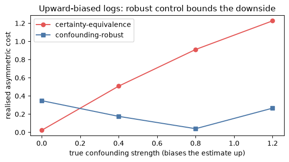
Pessimism is not free. The benchmark sweeps the true (unknown) confounding strength and reports the realised cost of both controllers. As in this log, every nonzero level biases the estimate upward. The robust controller bounds the worst-case cost and wins beyond a problem-dependent threshold, while paying a measurable premium near zero confounding (where its hedge costs more than it saves).
curve = confounding_robust_control_benchmark()
print(f"{'true confounding':>18} {'CE cost':>10} {'robust cost':>12}")
for conf, ce, rob in zip(curve.confounding_levels, curve.ce_costs, curve.robust_costs, strict=True):
    print(f"{conf:>18.1f} {ce:>10.3f} {rob:>12.3f}")
zero = list(curve.confounding_levels).index(0.0)
print(
    f"\nworst case over the sweep            : CE {curve.ce_worst_case:.3f}"
    f" -> robust {curve.robust_worst_case:.3f}"
)
print(f"savings at the log's confounding 0.8 : {curve.savings_at_target_pct:.0f}%")
print(
    f"premium when unconfounded            : robust {curve.robust_costs[zero]:.3f} vs CE "
    f"{curve.ce_costs[zero]:.3f} ({curve.unconfounded_premium_pct:.0f}% of the CE downside)"
)
  true confounding    CE cost  robust cost
               0.0      0.022        0.348
               0.4      0.508        0.175
               0.8      0.911        0.040
               1.2      1.226        0.265

worst case over the sweep            : CE 1.226 -> robust 0.348
savings at the log's confounding 0.8 : 96%
premium when unconfounded            : robust 0.348 vs CE 0.022 (27% of the CE downside)
# Optional plot (needs the `viz` group: uv sync --group viz). Text table above works without it.
try:
    import matplotlib.pyplot as plt

    fig, ax = plt.subplots(figsize=(6, 3.4))
    ax.plot(
        curve.confounding_levels,
        curve.ce_costs,
        "o-",
        color="#E45756",
        label="certainty-equivalence",
    )
    ax.plot(
        curve.confounding_levels,
        curve.robust_costs,
        "s-",
        color="#4C78A8",
        label="confounding-robust",
    )
    ax.set_xlabel("true confounding strength (biases the estimate up)")
    ax.set_ylabel("realised asymmetric cost")
    ax.set_title("Upward-biased logs: robust control bounds the downside")
    ax.legend()
    fig.tight_layout()
except ModuleNotFoundError:
    print("(install the `viz` group for the plot: uv sync --group viz)")
5 · When the hedge backfires, and what Gamma buys
Suppose instead that the past policy raised incentives when completions were hard to get, in bad weather say. The confounder then lowers completions, and the estimate is biased down. CE already over-incentivises, and the robust controller pushes the incentive further up. In the first table, which flips the sign of the sweep, the robust controller costs more than CE at every level: 0.906 against 0.416 at -0.8.
The second table goes back to the upward sweep and varies Gamma. A larger Gamma always costs more
without confounding: 0.138 at 1.5 and 0.565 at 4.0, against CE's 0.022. Of these five, the savings
at 0.8 are largest at the default Gamma = 2.5 (96 %) and fall on both sides (46 % at 1.5, 77 % at
4.0): a smaller Gamma hedges too little, a larger one overshoots the target. The analyst does not
know where the peak lies, so the 96 % in section 4 is close to a best case.
flipped = confounding_robust_control_benchmark(
    confounding_levels=(0.0, -0.4, -0.8, -1.2), target_confounding=-0.8
)
gammas = (1.5, 2.0, 2.5, 3.0, 4.0)
by_gamma = [confounding_robust_control_benchmark(sensitivity_gamma=g) for g in gammas]

print(f"{'true confounding':>18} {'CE cost':>10} {'robust cost':>12}   (biased down)")
rows = zip(flipped.confounding_levels, flipped.ce_costs, flipped.robust_costs, strict=True)
for conf, ce, rob in rows:
    print(f"{conf:>18.1f} {ce:>10.3f} {rob:>12.3f}")

print(f"\n{'Gamma':>6} {'savings at 0.8':>15} {'robust cost at 0':>17}")
for g, swept in zip(gammas, by_gamma, strict=True):
    print(f"{g:>6.1f} {swept.savings_at_target_pct:>14.0f}% {swept.robust_costs[zero]:>17.3f}")
  true confounding    CE cost  robust cost   (biased down)
               0.0      0.022        0.348
              -0.4      0.175        0.582
              -0.8      0.416        0.906
              -1.2      0.793        1.413

 Gamma  savings at 0.8  robust cost at 0
   1.5             46%             0.138
   2.0             85%             0.252
   2.5             96%             0.348
   3.0             89%             0.430
   4.0             77%             0.565
Honest caveats
Gammais the analyst's unfalsifiable sensitivity input; a single scalar aggregates over covariates. These methods robustify pessimism, they do not test for confounding.Gammacannot be tested, but it can be priced.benchmark_gammaexpresses it in units of the confounding an observed covariate carries, andnegative_control_gammareads a lower bound off an outcome the action cannot affect. This toy log has neither a covariate nor a negative control.- The CVaR-gap →
b_hatcalibration is a benchmark assumption, not a general consequence of the sensitivity model; the sign-identification constraintb_hat > D > 0must hold. - The sweep in section 4 is a synthetic observational task (the action follows the confounder); a genuine randomised switchback would reduce or remove the bias and is a natural experimental baseline.